Keywords: Parameter space, sample space, risk function
For noncommercial propose only. Some figures may be subject to copyright.
1. The formulation of decision theory
1.1 Elements in decision theory
1) Parameter space $\mathcal{\Theta}$ which will be a subset of $\mathbb{R}^d$ for some $d > 1$. It is the admissible set of unknown parameters in the decision problem. It is heuristic in this framework.
2) Sample space $\mathcal{X}$. The admissible set of X. For example, the sample space of stock price must be non-negative real number. The sample space is the possible value for observation.
3) A family of probability measure on the sample space $\mathcal{X}$. By convention, the probability measure can be written as $\{\mathbb{P}_{\theta}(x), x \in \mathcal{X}, \theta \in \mathcal{\Theta}\}$.
If we recall the definition of probability space, we can easily find out that the decision theory only consider a subspace of probability measure, which is parameterized by $\mathcal{\Theta}$.
4) Action space $\mathcal{A}$. This represents the set of all actions or decisions available to the experimenter. For a hypothesis testing problem, the action set is $\{“accept H_0”, “accept H_1”\}$. In an estimation problem, the action set $\mathcal{A} = \mathcal{\Theta}$.
5) A loss function $L: \mathcal{\Theta} \times A \xrightarrow{} \mathbb{R}$. The function implies the property of a specific action $\mathcal{a}$ when the parameters are $\mathcal{\Theta}$.
6) A set $\mathcal{D}$ of decision rules. An element d: $\mathcal{X} \xrightarrow{} \mathcal{D}$. Each point x in $\mathcal{X}$ is associated with a specific action $d(x) \in A$.
It is easily to connect this formulation with the reinforcement learning. Decision rule is a function mapping from the observation to action, which further implies that the risk function measure the coincidence of the parameter and the observation.
1.2 The definition of risk function
Risk function is $\mathcal{\Theta} \times \mathcal{D} \xrightarrow{} \mathbb{R}$. Note that the difference between the risk function and loss function is that the loss function measure the relationship of parameters and actions, which is deterministic, while the risk function is defined on the decision rule (since $x \in \mathcal{X}$ is a random variable). Of course, we can use other criterion besides expectation. However, expectation of loss function is the most reasonable one (we can further penalize the variance etc.). The risk function is trying to consider the influence of random variables. Heuristically, the risk function is defined as:
$$R(\theta, d) = \mathbb{E}_{\theta} L(\theta, d(X))$$
Note that the definition of risk function is based on the hypothesis of probability measure space. Once we determine the family of probability measure and decision rule, we can exactly determine the risk function. Risk function is similar to the concept of utility function in the Economics.
2. The criterion for a good decision rule
The final output of the decision theory is the decision rule, which is a function of $\mathcal{X} \xrightarrow{} \mathcal{A}$. We need to distinguish the decision rules, and find the better one.
2.1 Admissibility
Given two decision rules $d$ and $d^{‘}$, if $R(\theta, d) \le R(\theta, d^{\prime})$ for all $\theta \in \mathcal{\Theta}$, then $d$ strictly dominates $d^’$. If there exists a decision rule $d$ which strictly dominate decision rule $d^\prime$, then $d^\prime$ is said to be inadmissible (otherwise admissible). However, in practice, it is impossible to get an analytical solution of risk function. (A closed-form solution means we can extend the properties of risk function to any other point in the space). Therefore, it is very hard to determine if a decision rule is admissible or not.
2.2 Minimax decision rules
The maximum risk of a decision rule is defined as:
$MR(d) = \sup\limits_{\theta \in \mathcal{\Theta}}R(\theta, d)$
A decision rule is minimax if it minimizes the maximum risk:
$MR(d) \le MR(d^{\prime})$ for all decision rules $d^{\prime} \in D$
The idea behind the minimax decision rule is that we want to optimize the worst scenario. Note that minimax may not be the admissible decision rule and, apparently, may not be unique. However, if you are trying to choose the decision rule based on this criterion, you must follow the minimax idea.
Note that $\max_{\theta \in \Theta} = \min\limits_{d^\prime \in \mathcal{D}} \max\limits_{\theta \in \Theta} R(\theta, d^\prime)$
2.3 Unbiasedness
A decision rule $d$ is defined as unbiased if
$\mathbb{E}_{\theta} {L(\theta^{\prime}, d(X))} \ge \mathbb{E}_{\theta} {L(\theta, d(X))} $
Note that this notation is somehow confusing. $\mathbb{E}_{\theta} {L(\theta^{\prime}, d(X))} = \mathbb{E}_{X}(R(\theta, \delta)|\theta)$. Since $\delta$ is the function of $X$, we consider the connection of randomness of $X$. The decision here is
Note that this definition is quite tricky. We are calculating the expectation over the probability measure of $\mathcal{X}$, which is parameterized by $\theta$ (that’s why we use subscript $\theta$).
The unbiasedness is a criterion that does not depend on risk function only. The definition of unbiasedness depends on the parameters. This criterion makes the risk function self-consistent. However, the unbiasedness is somehow between a distraction and a total irrelevance. (原来不止我一个人这么想)
2.4 Bayes decision rule
We must specify a prior distribution, which represents our prior knowledge on the value of the parameter $\theta$, and is represented by a function $\pi(\theta), \theta \in \mathcal{\Theta}$. The prior distribution to be absolutely continuous, meaning that $\pi(\theta)$ is taken to be some probability density on $\mathcal{\Theta}$.
In the continuous case, the Bayes risk of a decision rule $d$ is defined to be $r(\pi, d) = \int_{\theta \in \mathcal{\Theta}}R(\theta, d)\pi(\theta)d\theta$. The decision rule $d$ is said to be a Bayes rule, with respect to a given prior $\pi(\dot)$, if it minimizes the Bayes risk, so that
$r(\pi, d) = \inf \limits_{d^\prime \in \mathcal{D}} r(\pi, d^\prime) = m_{\pi}$
Note that if the $\inf$ cannot be reached, we can further consider the $\epsilon$ decision rule, i.e.
$R(\pi, d_{\epsilon}) < m_{\pi} + \epsilon$. It is nothing but the definition of infimum with a more computable result.
2.5 Randomized decision rule
The Bayes decision rule consider the probability measure over $\theta$, while the randomized decision rule considers the probability measure over decision rules. Note that in the traditional mechanism, the probability measure is independent of the data. The risk function under the randomized decision rule can be written as:
$R(\theta, d^*) = \sum_{i=1}^l p_i R(\theta, d_i)$
If we consider the independent (wrt to data), it is easy to construct examples in which $d^{*}$ is formed by randomizing the rules $d_1, \dots, d_l$ but $\sup_{\theta} R(\theta, d^{*}) \le \sup_{\theta} R(\theta, d_i)$ for each i. The statement can be easily proved.
However, it is only holds for risk neutral decision maker. We also should consider the second order moment (the variance). We can formulate the metric like expected loss in this scenario.
It will be very interesting if we combine the Bayesian rules and randomized decision rule together.
3. A finite parameter space example
The discussion in the reference is not accurate. Based on the statement in the reference, we must construct an algebra over decision set. However, if we consider the risk function a measurable function, we can avoid the construction of an algebra.
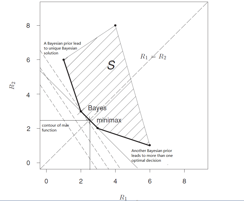
If we consider the limited number of parameters $\theta$, we can better understand the property of the decision set. Let’s consider a parameter space which is a finite set: $\mathcal{\Theta} = \{\theta_1, \theta_2 \dots, \theta_t\}$. Let’s consider a $t$ dimensional space. For a specific decision policy $d$ (including randomized policy), there is a specific generic point in this space, which can be written as $((R(\theta_1, d), R(\theta_2, d), \dots, R(\theta_3, d)))$. For any decision rule in set $\mathcal{D}$, let’s consider $d_1$ and $d_2$.
Since we can always find a randomized decision rule given a specific probability measure, the risk function space is convex over decision. For any $0<\lambda < 1$,
$\lambda((R(\theta_1, d_1), R(\theta_2, d_1), \dots, R(\theta_3, d_1))) + (1-\lambda)((R(\theta_1, d_1), R(\theta_2, d_1), \dots, R(\theta_3, d_1))) \xrightarrow{} d^*$, where $d^*$ is a randomized decision rule with probability measure $(\lambda, 1-\lambda)$. Therefore, we proved that risk function is convex over decision rules.
None of the decision rules can guarantee the uniqueness of the decision.
4. Finding minimax rules
A natural idea is to use the weak duality. However, we can hardly expect the inequality is tight for arbitrary function. Another idea is to find the minimax rules via Bayes principle. Note that the Bayes principle includes the minimum by definition.
Theorem 1:
If $\delta_n$ is Bayes with respect to prior $\pi_n(\cdot)$, and $r(\pi_n, \delta_n) \xrightarrow{} C$ as $n \xrightarrow{} \infty$, and if $R(\theta, \delta_0) \le C$ for all $\theta \in \Theta$, then $\delta_0$ is minimax.
Proof:
Suppose $\delta_0$ satisfies the conditions of the theorem but is not minimax. Then there exist $\delta^\prime$ such that $R(\theta, \delta^\prime) < C$ for every $\theta \in \Theta$. We can find an $\epsilon > 0$ that $R(\theta, \delta^\prime) < C - \epsilon$ for every $\theta \in \Theta$, which is equivalent to the statement that $r(\pi_n, \delta^\prime) < C - \epsilon$ for any n. According to the definition of convergence, we can further conclude that there exist an $n$ such that $r(\pi_n, \delta_n) \ge C - \epsilon / 2$. However, since we have proved that there exist another decision rule $r(\pi_n, \delta^\prime) < C - \epsilon$, then $\delta_n$ cannot be the Bayes rule. $\therefore$ $\delta_0$ must be the minimax. (Make it more adherent compared to the proof in the reference 1).
Theorem 2:
For any $\delta$, we have $\sup\limits_{\theta} R(\theta, \delta) = \sup\limits_{\Lambda (\theta)} \int R(\theta, \delta) d\Lambda(\theta)$
Proof:
We can easily prove that $\sup\limits_\theta R(\theta, \delta) \ge \sup\limits_{\Lambda (\theta)} \int R(\theta, \delta) d\Lambda(\theta)$. For the reverse of the equality, we can use a Dirac distribution and the definition of supremum to prove that.
Theorem 3:
Suppose $\Lambda(\theta)$ is a prior on $\theta$, and $\delta_\Lambda$ is the Bayes estimator under $\Lambda$. Suppose also that $r(\Lambda, \delta_\Lambda) = \sup\limits_\theta R(\theta,\delta_\Lambda)$. We can then conclude that:
1) $\delta_\Lambda$ is the minimax rules.
2) $\Lambda$ is least favorable.
Proof:
1) If $\delta_\Lambda$ is not the minimax rules. Then there exist $\delta^\prime$ such that $\sup\limits_{\theta} R(\theta, \delta^\prime) < \sup\limits_{\theta} R(\theta, \delta_\Lambda)$. Note that $r(\Lambda, \delta_\Lambda) = \sup\limits_\theta R(\theta,\delta_\Lambda)$ indicates that the $\delta_\Lambda$ is an equalizer decision rule ( $R(\theta, d)$ is the same for any $\theta \in \Theta$). Therefore, $r(\pi, \delta^\prime) < \sup\limits_\theta R(\theta,\delta_\Lambda)$ i.e. $\delta_\Lambda$ cannot be the Bayes rule. $\therefore$ $\delta_\Lambda$ is the minimax rules.
2) For an prior distribution $\pi^\prime$, the Bayes rule can be written as:
$r_{\pi^\prime} = \int R(\theta, \delta_{\pi^\prime}) \pi^\prime(\theta) d \theta \le \int R(\theta, \delta_{\pi}) \pi^\prime(\theta) d \theta \le \sup\limits_{\theta} R(\theta, \delta_{\pi}) = r_{\pi}$
The intuition is that we can always find the minimax via finding the least favorable prior distribution.
Reference
Essentials of Statistical inference. G.A. Young and R.L. Smith
EE378A Statistical Signal Processing Lecture 11: Minimax Decision Theory
Comments