Key words: convergence in distribution, Cauchy-Lorentz law, Domain of attraction, stable distribution, symmetric alpha-stable distribution ($\mathcal{S}\alpha \mathcal{S}$), Levy distribution
1. The exclusive properties of stable distributions
1.1 The definition of stable distributions-Invariance under addition
A random variables X is said to have a stable distribution $P(x) = Prob\{X \le x\}$ if for any $n \ge 2$, there is a positive number $c_n$ and a real number $d_n$ such that
$X_1 + X_2 + \dots + X_n \overset{d}{=} c_n X + d_n$
Note that the sum of i.i.d random variables becomes a random variable with a distribution of different form. However, for independent random variables with a common stable distribution, the sum obeys to a distribution of the same type, which differs from the original one only for a scaling and possibly for a shift. When $d_n = 0$, the distribution is called strictly stable.
It is known that the norming constants $c_n$ are of the form $c_n = n^{\frac{1}{\alpha}}$ with $0<\alpha \le 2$. The parameter $\alpha$ is called the characteristic exponent or the index of stability of the stable distribution.
By convention, we simply refer to $P_{\alpha}(x)$, $p_{\alpha}(x) = \frac{d P_{\alpha}(x)}{dx}$ and X as $\alpha-$stable distribution, density, random variable.
Alternative version: A random variable X is said to have a stable distribution if for any positive A random variable X is said to have a stable distribution if for any positive numbers A and B, there is a positive number C and a real number D such that
$A X_1 + B X_2 \overset{d}{=} CX + D$, where $X_1$ and $X_2$ are independent copies of $X$. Then there is a number $\alpha \in (0, 2])$, such that the number $C$ satisfies $C^{\alpha} = A^{\alpha} + B^{\alpha}$
This alternative version indicates that all linear combinations of i.i.d random variables obeying to a strictly stable distribution is a random variable with the same type of distribution.
If $-X$ has the same distribution. Of course, a symmetric stable distribution is necessarily strictly stable. ($AX_1 + BX_2 = CX + D$, $-AX_1 - BX_2 = -CX - D$ have the same distribution, which means $AX_1 + BX_2 = CX - D$ must hold. Therefore $D = -D, D = 0$)
1.2 Domain of attraction
Another (equivalent) definition states that stable distributions are the only distributions that can be obtained as limits of normalized sums of i.i.d. random variables. (可以用一组iid的随机变量的normalized summation依分布逼近)。
A random variable is said to have a domain of attraction, i.e. if there is a sequence of i.i.d. random variables and a sequence of positive numbers $\{\gamma_n\}$ and real numbers $\{\delta_n\}$, such that
$\frac{Y_1 + Y_2 + \dots + Y_n}{\gamma_n} + \delta_n \overset{d}{\xrightarrow{}} X$
Note that for convergence in distribution does not indicate the convergence in density function. For example, for the probability density function $f_n(x) = (1 - cos(2\pi n x)) 1_{x \in (0, 1)}$, the distribution converge to uniform distribution but the density function is not equal to the density function of uniform distribution over $(0, 1)$ a.s.
A random variable with domain of attraction is the sufficient and necessary condition for the stable distribution.
Note that if $X$ is Gaussian and the $Y_i$’s are i.i.d. with finite variance, then the domain of attraction is the statement of the ordinary CLT.
The domain of attraction of $X$ is said normal when $\gamma_n = n^{\frac{1}{\alpha}}$; In general, $\gamma_n = n^{\frac{1}{\alpha}}h(n)$, where $h(x)$ is a slow varying function at infinity. Note that we call a measurable positive function $a(y)$, defined in a right neighborhood of zero, slowly varying at zero if $\frac{a(cy)}{a(y)} \xrightarrow{} 1$ with y $\xrightarrow{} 0$ for every $c>0$. With the same logic we can define the slowly varying at infinity.
Note that 1.1 can derive 1.2, while 1.2 can derive 1.1 as well.
1.3 Canonical forms for the characteristic function
Another definition specifies the canonical form that the characteristic function of a stable distribution of index $\alpha$ must have. This condition implies the properties of cf, which will be useful in the CLT. The canonical forms reads
$\hat{p}_{\alpha}(\kappa; \theta) \overset{\Delta}{=} exp\{-|\kappa|^\alpha e^{i(\text{sign} \kappa)\theta \pi/2}\}$
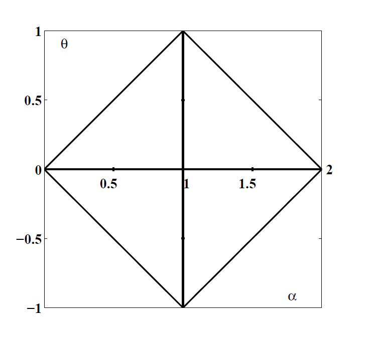
$\theta$ is called asymmetric parameter. The domain is restricted to the following region (depending on $\alpha$). For $ 0<\alpha\le 2$, $|\theta| \le \min(\alpha, 2-\alpha)$. The region is called Feller-Takayasu diamond.
A more common form of cf reads:
$\varphi(t; \alpha, \beta, c, \mu) = \text{exp}(it\mu-|ct|^\alpha(1-i\beta \text{sgn}(t)\Phi))$, where $\text{t}$ is the sign of t, and $\Phi = \tan(\frac{\pi \alpha}{2})$ when $\alpha \neq 1$, and $-\frac{2}{\pi} \text{log}|t|$ when $\alpha=1$. If $\mu = 0$, then the distribution is strictly stable.
Note that when $\beta = 0$, the cf can be written as:
$\varphi(t; \alpha, \beta, c, \mu) = \text{exp}(it\mu-|ct|^\alpha)$
We can further notice that the distribution is symmetric over $\mu$ (Remark: $\varphi(-x)\varphi(x) \in \mathbb{R}$). Therefore, when $\beta$ is zero, we call the distribution like this symmetric alpha-stable distribution, often abbreviated $\mathcal{S}\alpha \mathcal{S}$. $\beta \in [-1, 1]$ is also called skewness parameter.
All the distribution with the characteristic functions defined in 1.3 have the properties mentioned in 1.1 and 1.2 (sufficiently and necessarily).
2. Example
2.1 Gaussian Law
The characteristic exponent of Gaussian Law is $\frac{1}{2}$. Note that:
$X_1 + X_2 + \dots + X_n \sim N(nu, n\sigma^2)$ which can be written to $\sqrt{n}X + (n - \sqrt{n})\mu$. If $\mu = 0$, then X is strictly stable. Noteworthy observation is that the increment rate of variance is at least $\sqrt{n}$.
2.2 Cauchy-Lorentz
The probability density function of Cauchy-Lorentz distribution can be written as:
$f(x; x_0, \gamma) = \frac{1}{\pi \gamma}[\frac{\gamma^2}{(x - x_0)^2 + \gamma^2}]$.
The cumulative distribution function can be written as:
$F(x; x_0, \gamma) = \frac{1}{\pi} arctan(\frac{x - x_0}{\gamma}) + \frac{1}{2}$.
The distribution of the summation of random variables can be analytically solved by the characteristic function.
The cf of Cauchy distribution can be written as $e^{\gamma |k|}$. The summation of n iid random variables can be written as $e^{n\gamma|k|}$, which indicate that the index of Cauchy-Lorentz distribution is 1.
Reference
- B.V. Gnedenko, A.N. Kolmogorov, “Limit distributions for sums of independent random variables” , Addison-Wesley (1954) (Translated from Russian) MR0062975 Zbl 0056.36001
- LECTURE NOTES ON MATHEMATICAL PHYSICS Department of Physics, University of Bologna, Italy
Comments