Keywords: Neyman-Pearson Theorem, monotone likelihood ratio (MLR), LRT, Bayes factors, Frequentist VS Bayesian
1. Formulation
For a parameter space $\Theta$, and consider the hypothesis of the form:
$H_0: \theta \in \Theta_0$ vs. $H_1: \theta \in \Theta_1$
where $\Theta_0$ and $\Theta_1$ are two adjoint subsets of $\Theta$. Note that if $\Theta_0 = \{\theta_0\}$, then we call this simple hypothesis; otherwise composite hypothesis. (Watch out for nuisance parameters).
Note that when we are testing hypothesis based on the decision theorem, we have to calculate the risk function given a specific $\theta$. Since $\theta$ can at most in one of the hypothesis set, it is asymmetric between those two hypothesis.
The usual way is to construct a test statistic $t(X)$ and a critical region $C_\alpha$, then reject $H_0$ based on $X = x$ if and only if $t(x) \in C_\alpha$. The critical region must be chosen to satisfy $\text{Pr}_{\theta}\{t(X) \in C_\alpha\}$. The critical region must be chosen to satisfy:
$\text{Pr}_{\theta}\{t(X) \in C_{\alpha}\} \le \alpha $ for all $\theta \in \Theta_0$.
2. Power of testing
We need to consider if a test function $\phi$ is better then others. This criterion is call power of test. The definition of power function can be written as:
$w(\theta) = \text{Pr}\{Reject H_0\} = \mathbb{E}_{\theta} \{\phi(X)\}$
In most situation, the power of a test is the value of power function on alternative hypothesis, i.e. $w(\theta_1)$.
When we are considering a simple test, the power can be rephrased as the probability to reject the null hypothesis when the alternative hypothesis is true.
The idea of formulating a good test is to make $w(\theta)$ as large as possible on $\Theta_1$, while satisfying the constraint $w(\theta) \le \alpha$ for all $\theta \in \Theta_0$. (在保证原假设被拒绝的情况下,让critical region在备择假设下得measure尽可能得大)
In general, we will consider the following three scenarios.
1) Simple $H_0$ and simple $H_1$: use Neyman-Pearson Theorem to construct the best test.
2) Simple $H_0$ and composite $H_1$: use a representative $\theta$ in $\Theta_1$, and apply Neyman-Pearson theorem. This is called UMP (uniformly most powerful) test.
3) Composite $H_0$ and composite $H_1$: Harder.
Define the test function (loss function in Hypothesis test):
$\phi(x) = 1 \quad \text{if}\quad t(x) \in C_\alpha$ otherwise $0$.
Comments: The definition of power shows the logic of minimax. The setting is favorable to null hypothesis. If we can reject the null hypothesis in the worst situation, then we should be more confident to our decision. Therefore, people always choose the hypothesis they are more interested in to be the alternative hypothesis.
In conclusion, finding the most powerful testing function can be written as:
$\max w(\theta_1)$
$s.t. w(\theta_0) = \alpha $
2.1 Likelihood ratio test in simple test
Consider simple null hypothesis and simple alternative hypothesis. Define the likelihood ratio $\Lambda(x)$ by:
$\Lambda(x) = \frac{f(x; \theta_1)}{f(x;\theta_2)}$
, where $f$ is the probability density function or probability mass function. According to NP theorem, the best test of size $\alpha$ is of the form: reject $H_0$ when $\Lambda(X) > k_\alpha$.
The randomized test with test function $\phi_0$ is said to be a likelihood ratio test if it is of the form:
$\phi_0(x) = 1$ if $f_1(x) > Kf_0(x)$, $\gamma(x)$ if $f_1(x) = Kf_0(x)$, $0$ if $f_1(x) < Kf_0(x)$.
$0< \gamma(x) < 1$ and $K \ge 0$
Note: Test function is the loss function and decision rule in decision theory, while power is the risk function in the decision theory
2.2 Neyman-Pearson Theorem
Given the LRT define in 2.1, we can conclude that:
(a) (Optimality). For any K and $\gamma(x)$, the test $\phi_0$ has maximum power among all tests whose size are no greater than the size of $\phi_0$.
(b) (Existence). Given $\alpha \in (0, 1)$, there exist constants $K$ and $\gamma_0$ st the LRT defined by this K and $\gamma(x) = \gamma_0$ for all x has size exactly $\alpha$.
(c) (Uniqueness). If the test $\phi$ has size $\alpha$, and is maximum power amongst all possible tests of size $\alpha$, then $\phi$ is necessarily a likelihood ratio test, except possibly on a set of values of x which has probability 0 under $H_0$ and $H_1$. (给定$\alpha$和最强检验,则这个test function几乎处处是likelihood ratio test.)
Technical Condition: Probability density function or probability mass function of alternative hypothesis should Absolute continuous wrt the null hypothesis.
The proof follows common tricks used on decision theorem.
Proof:
(a) Let $\phi$ denote any test for $\mathbb{E}_{\theta_0} \phi(X) \le \mathbb{E}_{\theta_0} \phi_0(X)$ (any test function which has smaller size of critical region). Define $U(x) = [\phi_0(x) - \phi(x)][f_1(x) - kf_0(x)]$. Note that the state space of test function is 0 or 1 but with different domain. When $f_1(x) - Kf_0(x) > 0$, $\phi_0(x) = 1$, $U(x) \ge 0$. We also prove that $U(x) \ge 0$ when $f_1(x) - kf_0(x) < 0$. Therefore,
$0 \le \int [\phi_0 - \phi][f_1(x) - K f_0(x)] dx = \mathbb{E}_{\theta_1} \phi_0(X) - \mathbb{E}_{\theta_1} \phi(X) + K(\mathbb{E}_{\theta_0} \phi(X) - \mathbb{E}_{\theta_0} \phi_0(X))$
$\therefore \int [\phi_0 - \phi][f_1(x) - K f_0(x)] dx = \mathbb{E}_{\theta_1} \phi_0(X) - \mathbb{E}_{\theta_1} \phi(X) \ge 0$
The difference of power between two test function is always larger then K times the difference of size.
(b) Can be easily proved based on the fact that the cdf is right continuous, non-decreasing, and monotonous.
(c) Prove by contradiction. (读者自证真的不难)
2.3 Uniform most powerful (UMP) test and MLR
Just the same as the continuous and uniformly continuous, the UMP test is a global version of the most powerful test.
A uniformly most powerful or UMP test of size $\alpha$ is a test $\phi_0(\cdot)$ for which
(i) $\mathbb{E} \phi_0(X) \le \alpha$ for all $\theta \in \Theta_0$
(ii) given any other test $\phi(\cdot)$ for which $\mathbb{E}_{\theta} \phi(X) \le \alpha$ for all $\theta \in \Theta_0$, we have $\mathbb{E}_{\theta} \phi_0(X) \ge \mathbb{E}_{\theta} \phi (X)$.
For some family of parameters, the LRT is UMP in one-side testing problem. However, we can never assume LRT is UMP in the composite hypothesis. Such families are said to have monotone likelihood ratio or MLR.
Definition: The family of densities $\{f(x; \theta), \theta \in \Theta \in \mathbb{R}\}$ with real scalar parameter $\theta$ is said to be of monotone likelihood ratio if there exist a function t(x) such that the likelihood ratio
$\frac{f(x; \theta_1)}{x; \theta_0}$
is a non-decreasing function of $t(x)$ whenever $\theta_0 \le \theta_1$
Examples of MLR: $f(x; \theta) = c(\theta)h(x)e^{\theta \tau(x)}$ or the density distribution is irrelevant to $x$.
Theorem: Suppose $X$ has a distribution from a family of MLR with respect to a statistic $t(X)$, and that we wish to test $H_0 : \theta \le \theta_0$ against $H_1: \theta > \theta_0$. Suppose the distribution function of $t(X)$ is continuous.
(a) The test $\phi(x) = 1 $ if $t(x) > t_0$ or 0 otherwise is UMP among all test of size $\le \mathbb{E}_{\theta_0}[\phi_0(X)]$
(b) Given some $\alpha$, where $0<\alpha<1$, there exist some $t_0$ such that the test in $(a)$ has size exactly $\alpha$.
(easy to prove)
3. Bayes factor
3.1 Bayes factor in simple test
Suppose the prior probability that $H_0$ holds is $\pi_0$, and the prior probability that $H_1$ holds is $\pi_1$. The Bayes law leads to $\textbf{Pr}\{H_0 true | X= x\} = \frac{\pi_0 f_0(x)}{\pi_0 f_0(x) + \pi_1 f_1(x)}$. We can easily get that
$\frac{\textbf{Pr}(H_0 true | X = x)}{\textbf{Pr}(H_1 true | X = x)} = \frac{\pi_0 f_0(x)}{\pi_1 f_1(x)}$
We can conclude that:
Posterior Odds = Prior Odds $\times$ Bayes Factor
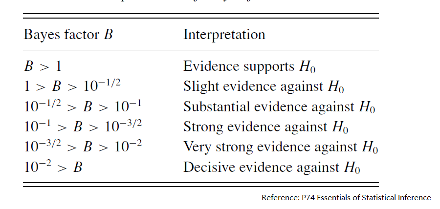
Note that the definition or Odds and Bayes Factor is null over alternative.
Interestingly, if we take the decision rule that reject $H_0$ if Bayes factor for some constant $k$ (and ignore randomized tests), then Bayes rule is exactly the same as the class of Neyman-Person rules.
3.2 Bayes factor in composite test
The Bayes Factor in composite test can be written as:
$B = \frac{\int_{\Theta_0} f(x; \theta) g_{\theta|\theta \in \Theta_0}(\theta) d\theta}{\int_{\Theta_1} f(x; \theta) g_{\theta|\theta \in \Theta_1}(\theta) d\theta}$
Note that in the hybrid mode like simple $H_0$ vs composite $H_1$, the conditional distribution will degenerate to Dirac distribution. For example, for $H_0 = \theta_0$ and $H_1 \neq \theta$ the Bayes Factor will therefore be written as:
$B = \frac{f(x; \theta_0)}{\int_{\Theta_1} f(x; \theta) g_{\theta|\theta \in \Theta_1}(\theta) d\theta}$
Note that the Bayes Factor allow the test conducted on different parameters set. For example, we have two models, i.e.
$p(x | M_i) = \int f(x; \theta_i, M_i) \pi_i(\theta_i) d\theta_i, i=1, 2$
The Bayes Factor is the ratio of these:
$B = \frac{p(x |M_1)}{p(x |M_2)}$
There is nothing about predictive, but a test about the prior distribution and model itself.
3.3 BIC
For large sample sizes n, we can approximate the Bayes Factor that:
$W = -2\log\frac{\sup_{\theta_1} f(x; \theta_1, M_1)}{\sup_{\theta_2} f(x; \theta_2, M_2)}$
$\Delta BIC = W - (p_2 - p _1)\log(n)$
$B \approx \exp(-\frac{1}{2} \Delta BIC)$.
Smaller $\Delta BIC$ provides more confidence about the null hypothesis, i.e. larger n do favor to more complicated model (with more parameters).
Note that we do not need know anything about the prior distribution about the parameters (only need to take the best situation).
3.4 Other improvement on Bayes Factor
(a) Find a reasonable approach to obtain the Bayes factor over a wide class of reasonable choice
(b) Partial Bayes factors
(c) Intrinsic Bayes factors
(d) fractional Bayes factors
Reference
Essentials of Statistics Inference
Comments