Keywords: Asymptotic distribution of estimators
1. The estimation of the mean value
1.1 Consistency
If $\{X_t\}$ is stationary with mean and $\mu$ and autocovariance function $\gamma(\cdot)$, then as $n \xrightarrow{} \infty$, $\text{Var}(\bar{X}_n) = \mathbb{E}(\bar{X}_n - \mu)^2 \xrightarrow{} 0$ if $\gamma(\cdot) \xrightarrow{} 0$,
and $n\mathbb{E}(\bar{X}_n - \mu)^2 \xrightarrow{} \sum_{n = -\infty}^{\infty} \gamma(h)$ if $\sum_{n = -\infty}^{\infty} |\gamma(h)| \le \infty$
Proof:
$n\text{Var}(\bar{X}_t) = \frac{1}{n} \sum_{i,j = 1}^{\infty} \text{Cov}(X_i, X_j) = \frac{1}{n} \sum_{i,j = 1}^{\infty} \gamma(h) = \sum_{|h| < n}(1 - \frac{|h|}{n})\gamma(h) \le \sum_{|h| < n}|\gamma(h)|$
Note that $\lim_{n \xrightarrow{} \infty}n^{-1}\sum_{|h| < n}|\gamma(h)| = 2 \lim_{n \xrightarrow{} \infty} |\gamma(n)| \xrightarrow{} 0$, hence $\text{Var}(\bar{X}_n) \xrightarrow{} 0$. If $\sum_{|h| < n}|\gamma(h)| < \infty$ then the dominate convergence theorem indicates that
$n\mathbb{E}(\bar{X}_n - \mu)^2 \xrightarrow{} \sum_{n = -\infty}^{\infty} \gamma(h)$
1.2 CLT for strictly stationary process
Lemma: Let $X_n$, $n = 1, 2,\dots$ and $Y_{nj}$, $j = 1, 2, \dots; n= 1, 2, \dots$ be random k-vectors such that
(i) $Y_{nj} \xrightarrow{d} Y_j$ as $n \xrightarrow{} \infty$
(ii) $Y_{j} \xrightarrow{d} Y$ as $j \xrightarrow{} \infty$
(iii) $\lim_{j \xrightarrow{} \infty}\text{limsup}_{n\xrightarrow{}\infty}P(|X_n - Y_{nj}| > \epsilon) = 0$ for every $\epsilon > 0$
Then $X_n \xrightarrow{d} Y$
Definition m-dependence: A strictly stationary sequence of random variables $\{X_t\}$ is said to be m-dependent if for each $t$, the two sets of random variables $\{X_j, j \le t\}$ and $\{X_j, j \ge t + m + 1\}$ are independent.
CLT for strictly stationary m-dependent sequences: If $\{X_t\}$ is a strictly stationary m-dependent sequence of random variables with mean zero and autocovariance function $\gamma(\cdot)$, and if $v_m = \gamma(0) + 2\sum_{j=1}^m \gamma(j) \neq = 0$ then
(i) $\lim_{n \xrightarrow{} \infty} n \text{Var}(\bar{X}_n) = v_m$
(ii) $\bar{X}_n$ is $AN(0, v_m/n)$
Proof:
(i) 易证。
(ii) 先通过m-dependent的独立性构造一个辅助随机变量序列,在证明$\{X_n\}$依分布收敛到这个辅助随机变量序列,这个方法值得借鉴。
For each integer k such that $k > 2m$, let $Y_{nk} = n^{-1/2} [(X_1 + X_2 + \dots + X_{k - m}) + (X_{k +1} + X_{k+2} + \dots + X_{2k - m}) + \dots + (X_{(r-1)k+1} + \dots + X_{rk-m})]$, where $r = [n/k]$. Note that $n^{1/2}Y_{nk}$ is a sum of r iid random variables each having mean zero and variance, $R_{k-m} = \text{Var}(X_1 + \dots + X_{k-m}) = \sum_{|j|< k-m}(k-m-|j|)\gamma(j)$. Apply CLT, we have $Y_{nk} \xrightarrow{} Y_{k}$, where $Y_k \sim N(0, k^{-1}R_{k-m})$. Moreover, note that $Y_{k} \xrightarrow{} Y$, where $Y \sim N(0, v_m)$. Then we need to prove that $\bar{X}_n$ converge to $Y_{nk}$ almost surely.
$\lim_{k \xrightarrow{} \infty} \text{limsup}_{n \xrightarrow{} \infty} P(|n^{1/2} \bar{X}_n - Y_{nk}| > \epsilon) = 0$ for every $\epsilon > 0$ (easy to prove).
1.3 Asymptotic normality
If $\{X_t\}$ is the stationary process,
$X_t = \mu + \sum_{j = -\infty}^{\infty} \varphi_{j}Z_{t-j}$, where $\{Z_t\} \sim IID(0, \sigma^2)$,
where $\sum_{j = -\infty}^{\infty}|\varphi_j| < \infty$ and $\sum_{-\infty}^{\infty} \varphi_{j} \neq 0$, then $\bar{X}_n \sim AN(\mu, n^{-1}v)$, where $v = \sum_{h=-\infty}^{\infty}\gamma(h) = \sigma^2(\sum_{j = -\infty}^{\infty} \varphi_j)^2$ (AN means asymptotic normal)
Proof: Define $X_{tm} = \mu + \sum_{j = -m}^m \varphi_{j}Z_{t-j}$ and $Y_{nm} = \bar{X}_{nm} = \frac{\sum_{i=1}^n X_{tm}}{n}$, $\text{Var}(n^{1/2}(\bar{X}_n - Y_{nm})) = n\text{Var}(n^{-1} \sum_{t=1}^n \sum_{|j|>m} \phi_{j}Z_{t-j}) \xrightarrow{}(\sum_{|j|>m}\varphi_j)^2\sigma^2$
2. The estimation of autocovariance function
2.1 Autocovariance function
$\gamma(h) = n^{-1} \sum_{t = 1}^{n - h} (X_t - \bar{X}_n)(X_{t + h} - \bar{X}_n), 0 \le h \le n - 1$. The reason why we do not use the unbiased estimator (you know what) is the we want to get an non-negative covariance matrix. For the estimated covariance matrix, we can write the $\hat{\Tau}_n$($\{\hat{\gamma}(i-j)\}$) as $\frac{1}{n}TT^{\prime}$. (Note that $TT^{\prime} = \{\sum_{k=1}T_{ik} T_{kj}\}$, recall the Einstein summation).$T = $ is a $(n \times 2n)$ matrix.
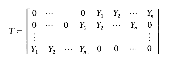
Recall that the sufficient and necessary condition of the non-negative matrix is that the there exist such a decomposition. Note that for any real vector $a$, we have $a^{\prime}\hat{\Tau}_n a = n^{-1}(a^{\prime}T)(a^{\prime}T)^\prime$
2.2 Autocorrelation function and asymptotic distribution
$\hat{\rho}(h) = \hat{\gamma}(h) / \hat{\gamma}(0)$
Theorem 2.2.1: If $\{X_t\}$ is the stationary process, $X_t - \mu = \sum_{j = -\infty}^{\infty} \varphi_j Z_{t - j}$, $Z_t \sim \text{IID}(0, \sigma^2)$, where $\sum_{j=-\infty}^{\infty}|\varphi_{j}| <\infty$ and $\mathbb{E}(Z_t^4) < \infty$, then for each $h \in \{1, 2, \dots\}$ we have $\hat{\rho}(h)$ is $\text{AN}(\rho(h), n^{-1}W)$, where $W$ is the covariance matrix whose $(i, j)$ element is given by Bartlett’s formula.
$w_{i,j} = \sum_{k=-\infty}^{\infty} \{\rho(k + i)\rho(k + j) + \rho(k-i)\rho(k + j) + 2\rho(i)\rho(j)\rho^2(k) - 2\rho(i)\rho(k)\rho(k + j) - 2 \rho(j)\rho(k)\rho(k + i)\} = \sum_{k= 1}^{\infty} \{\rho(k + i) + \rho(k-i) - 2\rho(i)\rho(k)\}\{\rho(k + j) + \rho(k-j) - 2\rho(j)\rho(k)\}$
Therefore, the asymptotic distribution of $n^{1/2}(\hat{\rho}(h) - \rho(h))$ is the same as that of the random vector $(Y_1, Y_2, \dots, Y_h)$, where $Y_i = \sum_{k=1}^{\infty}(\rho(k + i) + \rho(k -i) - 2\rho(i)\rho(k))N_k$
Theorem 2.2.2: If $\{X_t\}$ is the stationary process, $X_t - \mu = \sum_{j = -\infty}^{\infty} \varphi_j Z_{t - j}$, $Z_t \sim \text{IID}(0, \sigma^2)$, where $\sum_{j=-\infty}^{\infty}|\varphi_{j}|^2 <\infty$, then for each $h \in \{1, 2, \dots\}$ we have $\hat{\rho}(h)$ is $\text{AN}(\rho(h), n^{-1}W)$, where $W$ is the covariance matrix whose $(i, j)$ element is given by Bartlett’s formula.
Comments